230718 'HAND' http://farbe.li.tu-berlin.de/CEA_S.HTM or
http://color.li.tu-berlin.de/CEA_S.HTM.
For links to the chapter A
Colour Image Technology and Colour Management (2019), see
Content list of chapter A:
AEA_I in English or
AGA_I in German.
Summary of chapter A:
AEA_S in English or
AGA_S in German.
Example content part AEAI of some available parts AEAI to AEZI:
AEAI in English or
AGAI in German.
Example images part AEAS of all 26 parts AEAS to AEZS:
AEAS in English or
AGAS in German.
For links to the chapter B
Colour Vision and Colorimetry (2020), see
Content list of chapter B:
BEA_I in English or
BGA_I in German.
Summary of chapter B:
BEA_S in English or
BGA_S in German.
Example content part BEAI of some available parts BEAI to BEZI:
BEAI in English or
BGAI in German.
Example images part BEAS of all 26 parts BEAS to BEZS:
BEAS in English or
BGAS in German.
For links to the chapter C
Colour Spaces, Colour Differences, and Line Elements (2021), see
Content list of chapter C:
CEA_I in English or
CGA_I in German.
Summary of chapter C:
CEA_S in English or
CGA_S in German.
Example content part CEAI of some available parts CEAI to CEZI:
CEAI in English or
CGAI in German.
Example images part CEAS of all 26 parts CEAS to CEZS:
CEAS in English or
CGAS in German.
For links to the chapter D
Colour Appearance, Elementary Colours, and Metrics (2022), see
Content list of chapter D:
DEA_I in English or
DGA_I in German.
Summary of chapter D:
DEA_S in English or
DGA_S in German.
Example content part DEAI of some available parts DEAI to DEZI:
DEAI in English or
DGAI in German.
Example images part DEAS of all 26 parts DEAS to DEZS:
DEAS in English or
DGAS in German.
For links to the chapter E
Colour Metrics, Differences, and Appearance (2023),
under work, see
Content list of chapter E (links and file names use small letters):
eea_i in English or
ega_i in German.
Summary of chapter E:
eea_s in English or
ega_s in German.
Example content part eeaI of some available parts eeai to eezi:
eeai in English or
egai in German.
Example images part eeas of all 26 parts eeas to eezs:
eeas in English or
egas in German.
Project title: Colour and colour vision with Ostwald, device, and elementary colours -
Antagonistic colour-vision model TUBJND and properties for many applications
Chapter C: Colour Spaces, Colour Differences, and Line Elements (2021),
Main part CEA_S
Title: Mathematical relations of spaces and differences in both directions;
Threshold colour differences for different viewing situations;
Line elements for different viewing situations;
Colour spaces for different viewing situations;
Modifications of the CIELAB colour space and the CIELAB colour difference
for different viewing situations and applications.
1. Introduction and goals.
2. Colour differnce formula LABJND of CIE 230:2019
based on threshold data delta_Y.
3. Contrast and thresholds as function of the luminance L,
and of the tristimulus value Y.
4. Colour line elements and derivations for the description of
colour differences of adjacent and separate colours.
The following pages of the chapter
Colour spaces, colour differences, and line elementes
give an introduction with special images.
1. Introduction and goals
This part shows relations of the colour spaces and the colour differences
with line elements.
Mathematical relations of the colour spaces and the colour differences
with line elements shall be developed.
2. Colour difference formula LABJND of CIE 230:2019
based on threshold data delta_Y
This part includes information on threshold data delta_Y.
These data are used as basis for the colour difference formula LABJND of CIE 230:2019.
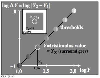
Figure 1: Visual threshold delta_Y of achromatic samples
in a grey surround with a white frame.
For the download of this figure in the VG-PDF format, see
CEA10-1N.PDF.
The figure shows that the threshold delta_Y
increases linear with Y. Therefore the so called
Weber-Fechner ratio Y/delta_Y
is constant within the range 10 <= Y <= 100.
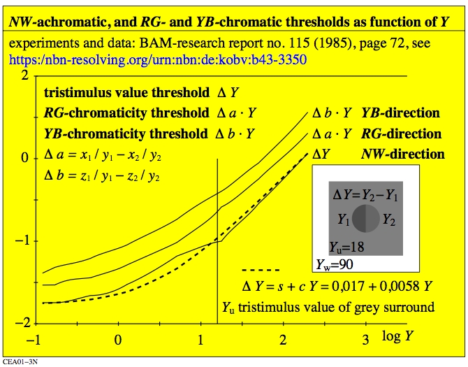
Figure 2: Visual threhold delta_Y of achromatic and chromatic samples
in a grey surround with a white frame.
For the download of this figure in the VG-PDF format, see
CEA01-3N.PDF.
The figure shows that the threshold delta_Y
increases approximately linear with Y. Therefore the so called
Weber-Fechner ratio Y/delta_Y
is approximately constant within the range 10 <= Y <= 100.
For the tristimulus values Y < 0,4 it is valid delta_Y=0,012.
For all values Y < 0,4 the two central field colours
appear as a uniform deep black.
The results in Fig. 2 are the basis of the colour-difference formula
LABJND for Just Noticeable Differences (JNDs) in CIE230:2019.
The performance of LABJND_PF is calculated in Table 9 and 11 of CIE 230
for the scope range 0 <= delta_E*ab <=2 of the CIELAB colour-difference formula,
and for the 8 available CIE datasets, see
http://files.cie.co.at/TC181_Datasets.zip.
The LABJND_PF colour difference formula shows the best performance for
5 out of 8 CIE datasets. CIELAB_PF, CMC_PF, and CIEDE2000_PF show the best performance
for one dataset. The abbreviation "_PF" stands for a "power function correction". This
correction is given for the five colour difference formulae
CIELAB, CMC, CIE94, CIEDE2000 and LABJND. The values of the calculated colour differences
decrease by the PF exponent for larger colour differences. This increases the performance
of each formula.
The comparison of the five formulae for large (LCD) and extra large (ELCD)
colour differences shows about the same performance for all formulae, see
YE370-7N.PDF.
It is recommended to compare the results for the scope range 5 < delta_E*ab < 199
of the CIE committee TC1-63. In 2016 the CIE TC1-63 members could not agree
to proceed with the draft WD11 for this CIE report on large colour differences,
for example based on this (unexpected?) result.
6. Contrast and threshold as function of luminance L
and tristimulus value Y.
This part includes information on the display or scene contrast between
white and black. This contrast is described by a ratio of the two reflections, or
the two tristimulus values, or the two luminance of white and black, for example
YW:YN=25:1.
The threshold contrast for just noticeable differences is described by the ratio
R/delta_R, or Y/delta_Y, or Ldelta_L.
oder Ldelta_L beschrieben.
The luminance L is proportional to the tristimulus value Y.
For surface colours the scene contrast YW:YN is often similar
to the visual threshold contrast Yu/delta_Yu (u=grey surround, German: Umfeld),
for example 25:1. The maximum visual threshold contrast is near 100:1.
This contrast decreases with the age of the observer.
The reason is the increasing stray light on the retina.

Figure 3: Contrast L/delta_L of achromatic samples
for five surround luminance.
For the download of this figure in the VG-PDF format, see
CEA10-7N.PDF.
Experimental results of Lingelbach [3] show the visual threshold contrast for
five different surround luminance. In a standard office the luminance is 142 cd/m^2
for the standard illumination 500 lux, and for
the standard White with the reflection R=0,90.
Fig. 3 shows approximately the contrast L/deltaL=25:1. In the experimental case
for surround with the luminance Lu=100 appears white. The data describe the threshold
for a long time adaptation (t > 600s) on a surround luminance Lu and the short time
presentation (t=0,1s) of a central field difference delta_L.
The curve shape is approximately a Gauß function.
The difference delta_L decreases for smaller and larger central field luminance
compared to the surround luminance.
However, if the presentation time increases to about t=2s, then the Weber-Fechner ratio
L/delta_L
is approximately constant according to the Weber-Fechner law.
This ratio still decreases to both sides of the surround luminance and more towards black.
However, it is approximately constant for achromatic surface colours
in the tristimulus value range 0,2Yu <= Y <= 5Yu.

Figure 4: Contrast values L/delta_L and three other plot possibilities
as function of L.
For the download of this figure in the VG-PDF format, see
CEA01-7N.PDF.
In Fig. 4 the central field lightness L* is calculated from
experimental threshold results delta_L by integration.
According to Schroedinger and Stiles [1] the function L*
is called the line element of the achromatic colour vision.
The experimental threshold results can be calculated from
L* by derivation.
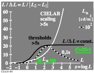
Figure 5: Ratio L/delta_L
as function of L for the lightness L*CIELAB and L*th (schematic).
For the download of this figure in the VG-PDF format, see
CEA10-8N.PDF.
In Fig. 5 the derivation of the lightness L*CIELAB
gives the function L/delta_L (in white). This is very different to the
approximately constant Weber-Fechner ratio L/delta_L (in black).
The normalisation of the lightness L*JND for adjacent samples
from the Weber-Fechner ratio will be described further with Fig. 16.
In a vision model Richter (2006) shows many connections for scaling
of separated colours according to the Stevens law,
and the threshold (JND) for adjacent colours
according to the Weber-Fechner law on a grey surround, see
BAMAT.PDF.
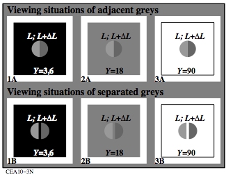
Figure 6: Viewing situtations of adjacent and separated samples.
For the download of this figure in the VG-PDF format, see
CEA10-3N.
In Fig. 6 grey samples are shown as two adjacent (top) or separated (botom) samples.
For surface colours in the range 4 < Y < 100 the
tristimulus-value differences delta_Y or the luminance differences
delta_L depend on the black, or the grey, or the white surround.
The following Fig. 17 shows a larger dependance of the threshold on the distance or
the separation of the two samples.
This separation effect is for example applied in the automotive industry.
Different parts of a car which may be painted at different locations
are often separated by small gaps of for example 2 mm. Then the
visual detection of small colour differences is reduced by about a factor 3.
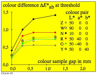
Figure 7: Colour difference in the lightness direction as function of the sample distance.
For the download of this figure in the VG-PDF format, see
CEA10-5N.PDF.
The figure shows six different colours with their CIELAB data L*a*b*.
The threshold was measured for adjacent and separated samples. One sample was lighter.
The threshold increases with the sample distance or the gap between the samples.
Already a gap of 2 mm in a viewing distance of 50 cm increases the colour difference
at threshold by about a factor 3. For larger sample gaps the colour difference
is constant.
The CIELAB lightness L* is not directly normalised to describe the threshold
of separated colours.
However, in many applications a lightness difference of delta_L*=1
is assumed as the threshold for separated colours on a grey surround.
Then the threshold is by a factor 3 smaller for adjacent compared to separated colours
on the same grey background. This is also shown in Fig. 15
The L* functions and the derivation functions can be normalised with the experimental
results of Fig. 17. In Fig. 15 both delta_Y threshold values are normalised at the
surround luminance Lu. This delta_Yu-threshold value is by about a factor 3 smaller
for separated colours compared to adjacent colours.
Several available datasets of CIE TC1-81 have shown approximately a threshold
delta_L*JND=0,30 for adjacent colours. However, Members of CIE TC1-81 could not agree
to recommend this threshold for adjacent colours. Therefore in CIE 230:2019
further research is recommended. However, in addition for example Fig. 17 shows that the
threshold is by a factor three smaller for adjacent colours compared to separated colours.
References:
[1] Stiles, W. S. (and E Schroedinger) (1972), The line element in colour theory:
a historical review, p. 1-25, in Color metrics, AIC/Holland, TNO Soesterberg.
[2] Seim, T. and A. Valberg (2015), A neurophysiological based analysis of
lightness and brightness perception, CR&A, 26 pages, This paper includes important
threshold data for adjacent colours, and for different presentation times,
and different adaptation luminance for improved colour vision models.
[3] Haberich, F. J. and B. Lingelbach, Psychophysical measurement concerning
the range of visual perception, Pflügers Archiv 1980; 386, 141-146.
[4] Avramopoulos, D. (1989), Leuchtdichte-Unterscheidungsvermögen von unbunten
und bunten Infeldfarben für kurz- und langzeitige Leuchtdichte-Unterschiede
(Luminance discrimination of achromatic and chromatic central fields for short and
long term luminance differences], see
UE.HTM.
[5] Richter, K., (1996), Computergrafik und Farbmetrik [computer graphic and
colorimetry], VDE-Verlag, Berlin - Offenbach, 288 pages, see
BUA4BF.PDF.
[6] Richter, K., (2012), Colour and colour vision - Elementary colours
in colour image technology, 72 pages, Berlin University of technology, section
lighting technology, with about 100 colour figures, see
http://standards.iso.org/iso/9241/306/ed-2/index.html.
[7] CIE 230:219, Validity of formulae for prediction small colour differences,
developed by CIE TC1-81 with the chairman: Klaus Richter, see for a summary at
http://www.cie.co.at/publications/validity-formulae-predicting-small-colour-differences.
Summary of this part
The luminance range in offices with paper and display applications is similar according to
ISO 9241-306. In this luminance range with 0,2Lu < L < 5Lu
the Weber-Fechner ratio L/delta_L is approximately constant.
This range corresponds to the normalised reflection range 0,2 < R1 < 5,0 in Fig. 9
or the reflection 0,04 < R <1,00 in Fig. 2. In this range the threshold is
by a factor 3 smaller for adjacent colours compared to separated colours,
see figures 16 and 17.
4. Colour line elements and deviations for the description
of colour differences of adjacent and separated colours

Figure 8: Approximation of the lightness L*CIELAB by L*Z for a grey surround;
Lightness L*W for a white and L*N for a black surround.
For the download of this figure in the VG-PDF format, see
CEA10-4N.PDF.
The figure shows different scaling funktions for the surrounds White W, mean Grey Z,
and Black N. Power functions with different exponents between
0,5 < k < 0,33 are used in applications.
Often separated colours are viewed on a grey surround. They appear
equally spaced in lightness, if the differences delta_L* are equal.
This is for example fulfilled for a 16 step grey scale with the lightness
L*CIELAB=15, 20, 25, ..., 85, 90.
In Figure 17 the calculated colour difference is about three times smaller
for adjacent compared to separated colours.
Figure 9: Viewing situations of adjacent and separated colours.
For the download of this figure in the VG-PDF format, see
CEA10-3N.PDF.
This figure shows in all smaller figures a mean grey surround. The figures 1A to 3A
show adjacent samples and the figures 1B to 3B separated samples. There are three
possibilities to specified the grey samples. One can use: the reflection R,
the tristimulus value Y, or the luminance L. Most of the users prefer
for grey colours the reflection R, which is also preferred in the following.
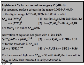
Figure 10: Lightness L*Z of separated greys in a main grey surround Z
For the download of this figure in the VG-PDF format, see
CEA11-1N.PDF.
The figure uses the lightness L*Z of the sRGB colour space
according to IEC 61966-2-1, compare L*Z in Fig. 40. Two normalisation of the
reflection are given in equation [1] and [2] in the Fig. 42. The first one is widely used
in colorimetry. However, the second one is preferred in the following
and based on colour physiology. The antagonistic colour vision model
is based on antagonistic signals White W and Black N with Grey Z
in the middle.
One must consider that mean grey is defined by the logarithmic mean of the
Reflection RW=0,9 of White and RN=0,036 of Black. If the reflection
is normalised to R1 = R/0,20 then R1W is five times larger compared
to R1Z and R1N is five times smaller compared to R1Z.
Therefore the logarithmic values are:
log(R1W) = log 5
log(R1Z) = 0
log(R1N) = log (1/5) = - log 5.
The logarithmic mean is:
log R1Z = 0,5 [ log(R1W) + log(R1N) = 0,5 [ log 5 + (- log 5)] = 0.
Equation [4] in the Fig. 42 describes the experimental result of Fig. 12.
It is approximately valid for adjacent samples:
delta_R/R^0,14 = const.
This is approximately the Weber-Fechner ratio:
delta_R/R = const.

Figure 11: Lightness L*JND of adjacent greys in a main grey surround Z
For the download of this figure in the VG-PDF format, see
CEA11-2N.PDF.
This figure uses the experimental exponent k=0,14 which is
by a factor three different to the exponent
k=0,42 in Figure 10. Therefore the lightness for adjacent colours is
different to the lightness of separated colours.
Mathematically the slope is defined by different exponents of the L* functions.
Further the L* functions differ by different scaling constants.
In experiments for the surround the slope can be determined
by a normalisation to the surround values. The scaling constant can be determined
by an appropriate normalisation to the reflection threshold at the surround.
The lightness function L* is called the line element of the lightness differences
at threshold. Equation [4] in Fig. 11 defines the values delta_R as function of
R. The values delta_R can be measured in visual threshold experiments
with the viewing situation 1A in Fig. 9. With these experimental
values a function for the lightness L* can be determined.
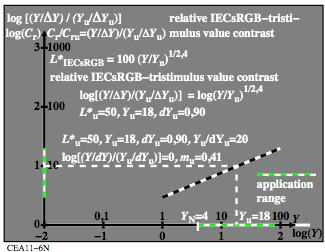
Figure 12: Line element and derivation of the lightness formula
L*IECsRGB
For the download of this figure in the VG-PDF format, see
CEA11-6N.PDF.
The lightness L*IECsRGB is an approximation of the lightness
L*CIELAB, compare Fig. 8. This lightness is intended for separated
samples on a mean grey surround.
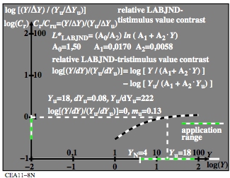
Figure 13: Lightness L*LABJND of adjacent greys in a mean grey surround Z;
Use in the colour difference formula LABJND of CIE 230
For the download of this figure in the VG-PDF format, see
CEA11-8N.PDF.
The lightness formula L*LABJND in Fig. 13 describes the
threshold for adjacent greys on a mean grey surround Z.
This lightness formula uses three constants A0, A1 and A2.
The formula was developed by integration of threshold results.
A BAM-research report of Richter (1985) describes the experimental thresholds
delta_Y as function of Y for achromatic and special
chromatic colour series. These BAM results are shown in Fig. 2.
The LABJND colour-difference formula of 1985 uses these results with the constants
A0, A1, and A2. The LABJND colour difference formula is used in CIE 230:2019.
The performance of the five colour difference formulae CIELAB, CMC, CIE94, CIEDE2000,
and LABJND is evaluated.
According to Table 9 and 11 of CIE 230, the LABJND_PF formula shows the best performance
for 5 out of 8 CIE datasets. CIELAB_PF, CMC_PF, and CIEDE2000_PF gives
the best performance for one of the 8 datasets, see the datasets
TC181_datasets.zip
The best performance of the five colour difference formulae is one advantage of LABJND.
The probably more important advantage is the line element
L*LABJND as function of Y. This is the calculated
lightness in Fig. 13 by integration of the threshold results.
If this integration is also possible for the antagonistic directions R-G and Y-B
with the BAM and other data, then probably two new colour spaces
for colour appearance are created. The two exponents k=0,42 and k=0,14 for
separated and adjacent colours in Fig. 10 and 11 may be used to calculate the thresholds
for these two viewing situations.
Other constants A0, A1, and A2 may be needed:
1. for black and white surrounds, compare Fig. 6 and 8,
2. different luminance adaptations, compare Fig. 4, and
3. different viewing times, compare Fig. 5, and
4. different chromatic adaptations, compare left and right in
BGH5L0NP.PDF.
It is intended to reach some of these goals by integration
of threshold data in a new
Part C: Colour Appearance, Elemenmtary Colours, and Colour Differences.
Further remarks
CIE 230:219 includes only the threshold function delta_Y as function of Y
for the definition of the LABJND-colour difference formula.
CIE 230 includes NOT the corresponding line element L*JND of Fig. 13.
For this unanimity was required by all TC1-81 members, and this was not possible.
The missing corresponding colour appearance space is a larger disadvantage
of the colour difference formulae CMC, CIE94, and CIEDE2000.
This advantage of the CIELAB space may be reached also with LAB2JND by integration
of the BAM and other threshold results.
For more equations calculated from the lightness L*LABJND, see for example
BEU41-7N.PDF.
In CIE 230 the chromatic values (A, B) of LABJND have been used. In future
calculations with the more visual chromatic values (A2, B2)
of LAB2JND may lead to an increase of the performance.

Figure 14: Line element and derivation of the lightness
L*IECsRGBJND
For the download of this figure in the VG-PDF format, see
CEA11-7N.PDF.
The lightness L*IECsRGBJND is intended to describe the threshold
for adjacent samples on a mean grey surround. For this aim the constants of the
lightness L*IECsRGB for separated samples are modified for
adjacent samples.

Figure 15: Colour attribute chromaticness C* and
achromaticness A*
For the download of this figure in the VG-PDF format, see
CEA11-5N.PDF.
The lightness L*CIELAB is intended to describe the threshold
for separated samples on a mean grey surround. The slope mu=0,33 shows some
difference compared to the slope mu=0,42 of the lightness L*IECsRGB.
Summary of this part:
The lightness is for separated and adjacent samples different.
It is usually valid
1. the lightness differences can be calculated from the lightness function
by mathematical derivation.
2. the lightness function can be calculated from the lightness differences
by mathematical integration.
3. For surface colours logarithmic properties of the lightness functions
can be approximated by exponential functions in the limited range of
R, Y or L.
This web site is under work since 2021.
In future the figures and the text will be improved depending on new results.
-------
For the TUB start site (not archive), see
index.html in English, or
indexDE.html in German.
For the TUB archive site (2000-2009) of the BAM server
"www.ps.bam.de" (2000-2018)
about colour test charts, colorimetric calculations, standards,
and publications, see
indexAE.html in English,
indexAG.html in German.
For similar Information of the BAM server "www.ps.bam.de"
from the WBM server (WayBackMachine)
https://web.archive.org/web/20090402212108/http://www.ps.bam.de/index.html